Leveraging Time Series Prediction to Reduce False Positives in Anomaly Detection Models
Welcome to our series of research-focused topics from the BlackBerry Cylance Data Science Team. In our horizon-based model, our Data Science team completes early research to solve cybersecurity-focused problems, expanding the capabilities of our Cylance portfolio and the customers we protect around the world.
In this post, we will discuss how to reduce false positives in anomaly detection models using time series to predict expected vs unexpected anomalies. We will use the gold standard for time series predictions, the ARIMA (Autoregressive Integrated Moving Average) model, and test with Lag-Llama, a recently published generative model for this task
Anomaly Detection Models in Cybersecurity
The goal of anomaly detection models in cybersecurity is to accurately identify malicious anomalies while minimizing false positives. Anomalies themselves do not necessarily mean something is good or bad but rather that it varies from what we would expect based on typical trends. Thus, most anomaly detection ML models struggle, producing too many false positives that require manual investigation.
In this blog, we will discuss a practical approach. By leveraging time series prediction techniques, we can help reduce false positives identified by anomaly detection models without compromising true positives. This methodology, demonstrated with real-world examples, can be generally applied in any anomaly model.
Forecasting Anomalies
While point and collective anomaly detection are common (isolating outliers and identifying unusual trends in groups), contextual anomalies are trickier. These anomalies might not be malicious but do appear unusual in specific situations. For example, high CPU usage during peak business hours is likely normal, but the same thing during off-hours is anomalous.
The key question here is: If we track historical anomaly detections, can we predict them in advance? This allows us to potentially suppress expected anomalies, likely reducing false positives from contextual variations and then focus on truly malicious activity.
Stationarity and Non-Stationarity of Anomalies
Time-series data is considered stationary if its statistical properties (mean, variance, autocorrelation) remain constant over time. Conversely, non-stationary data exhibits trends, seasonality, or changes in variance over time. Many anomaly detection algorithms, like Isolation Forest and Random Forest, assume stationarity. Non-stationary patterns in the data can lead to misinterpretations and false positives. Thus, most anomaly detection models struggle with non-stationary data.
Experimental Setup
We trained a network anomaly model to identify anomalous network behavior using NetFlow data. The method of the network anomaly model is not in scope for this blog. However, the approach of learned in-trend and out-of-trend anomaly can be a basis for pruning model output, or be an input to the base anomaly model, for better prediction. The question is if network anomalies themselves were observed as time-sequenced non-stationary events, can we discern a normal anomalous pattern?
Baseline with ARIMA (Auto Regressive Integrated Moving Average)
Imagine you're running a bakery and want to predict how many cupcakes you'll sell next week. ARIMA can help you with this by considering three key factors:
Past Sales (AR)
How much do your daily cupcake sales depend on the sales from the previous few days (similar to the "p" value)? Did you have a big promotion last week that might affect sales this week? It’s the number of lag observations in the trend. As in, how many past values are we looking at to make a forecast? It is a linear regression based on the number of past values.
Seasonal Trends (I)
Do you typically sell more cupcakes during holidays or weekends? This is the "d" value, which evens out these trends by looking at differences in sales between days including the number of times the raw observations are differenced. The number of differences may need to be increased if the moving average is not stationary. To determine if the series is stationary or not, we typically use the Augmented Dickey Fuller Test (ADF). For the ADF test, if the p-value is less than the significance level of 0.05 then we say the series is stationary.
Random Fluctuations (MA)
Sometimes, unexpected sales spikes occur due to a local event or a bad batch that gets discounted. The "q" value considers these short-term changes in sales to improve the accuracy of your predictions.
ARIMA considers recent trends and random bumps for predictions. In this case, "p" looks at past events, "d" removes trends, and "q" smooths out bumps. To consider seasonal fluctuations, one month of data may not be sufficient. A larger range would be required. For seasonal patterns, there is S-ARIMA (Seasonal ARIMA) that can be incorporated as well.
Using ARIMA to Filter Isolation Forest Anomalies
As proof of concept, we built upon an Isolation Forest anomaly detection model to add a time series filtering step. Isolation Forest is an unsupervised anomaly detection algorithm commonly used to detect outliers in datasets. However, it often produces many false positives in practice.
We first trained an Isolation Forest model on 14 days of network event data to detect anomalies. We then used the labeled output to incrementally train an ARIMA time series model.
We grouped the anomalous events detected each day by 5-minute time windows and trained the ARIMA model on this aggregated time series data. We then predicted anomalies for the 15th day using both models. Any events flagged as anomalous by Isolation Forest but predicted as normal by ARIMA were considered potential false positives. By comparing the two models' outputs, we were able to filter out anomalies that did not follow expected time series patterns, thus reducing false alerts.
ARIMA Model Configuration
Next, we set about minimizing Akaike Information Criterion (AIC), including the optimal values time window of interest for (p, d, q) = (3,1,2). The learning task here is optimize AIC for p, d and q for the window of data that needs to be forecast.
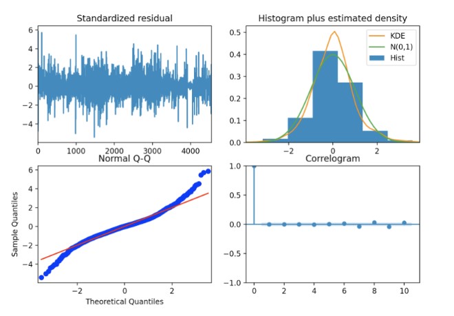
After applying power transformation to the data, we observe (below) that our model fits the data quite well. Residuals are centered around zero, indicating no bias in the data. Random scatter around zero indicates the model has captured the main trends and variations well. The consistent variance of residuals around zero suggests stability across all data points.
However, in the Q-Q plot we notice not all points are on the trend line. Points curve away from diagonal tails (top and bottom), suggesting the model might be underestimating the variance of the residuals in the tails. This explains the outliers or heavy-tailed distributions in our data.
Correlogram shows zero centered with -2, +2 range implying weak linear relationship with its past values as most lags (time steps). Overall, it appears that ARIMA may not be the best for this type of time series data.
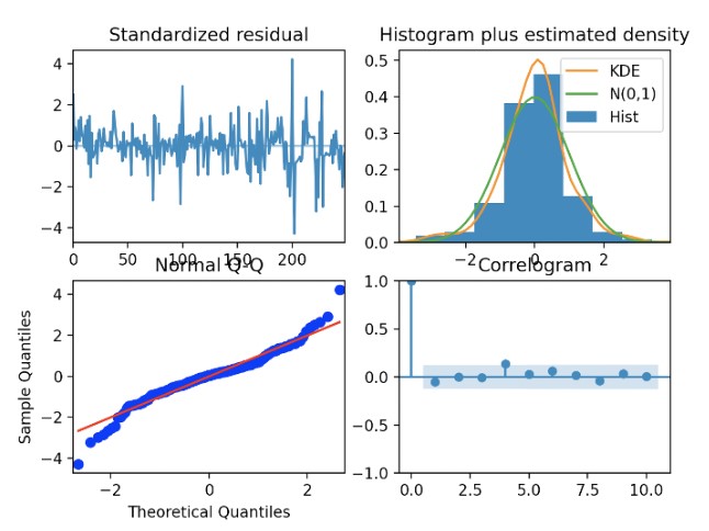
By fine-tuning the time window and p-value further, we arrive at slightly better results (below). With a time window of one hour and re-learning p, d, and q values in the sliding window, we see less tail-heavy divergence in the residual quantile plots and a tighter around-zero correlogram.
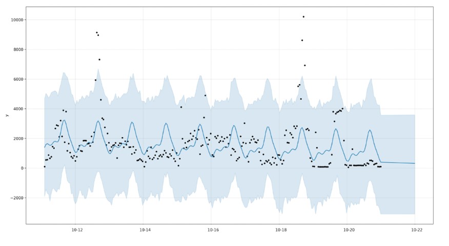
Below, the plot of predicted ranges shows the captured anomalies as black dots. The black dots, representing the test data, show no apparent trend. However, when we apply a time-series forecast, we can see captured trends and ranges.
In this example, we are applying ARIMA with a power transformation and a one hour window identified trend range in anomaly data. While this demonstrates the effectiveness of using time series prediction to filter out non-stationary anomalies flagged by Random Forest, the normal operating range is a bit large. This has the potential of missing a few true positive anomalies.
Lag-Llama LLM Time-Series Forecasting
In a recent paper on time series forecasting, researchers used a decoder-only transformer architecture with lags as covariates. It is pre-trained on a diverse corpus of time series data from various domains. Llama, an LLM, processes sequences by tokenizing them with covariates, then utilizes pre-normalization (RMSNorm, Rotary positional encoding) to improve attention mechanisms for better sequence understanding.
For predictions, it takes features from the time series and generates a distribution through a greedy autoregressive decoding. This allows for the simulation of multiple future trajectories up to the prediction horizon.
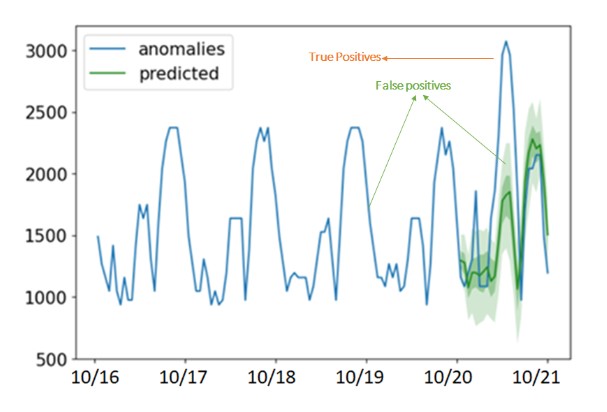
When fine-tuned on a small subset of this anomaly dataset, Lag-Llama does a good enough job forecasting (below) over the same one hour context window and for the next 12 hours.
Conclusion
We can use time series prediction to reduce false positives in anomaly detection. By considering stationarity and adjusting ARIMA parameters, we can improve accuracy and efficiency. The new Lag-LLAMA offers a powerful alternative forecasting approach as combining anomaly detection with time series prediction builds more robust and reliable solutions for better decision-making.
For similar articles and news delivered straight to your inbox, subscribe to the BlackBerry Blog.
About Rejish PC
Rejish PC is a Distinguished Software Architect at BlackBerry.

About The BlackBerry Cylance Data Science and Machine Learning Team
The BlackBerry Cylance Data Science and Machine Learning research team consists of experts in a variety of fields. With machine learning at the heart of all of BlackBerry’s cybersecurity products, the Data Science Research team is a critical, highly visible, and high-impact team within the company. The team brings together experts from machine learning, stats, computer science, computer security, and various applied sciences, with backgrounds including deep learning, Bayesian statistics, time-series modeling, generative modeling, topology, scalable data processing, and software engineering.
What we do:
- Invent novel machine-learning techniques to tackle important problems in computer security
- Write code that scales to very large datasets, often with millions of dimensions and billions of attributes
- Discover ways to strengthen machine learning models against adversarial attacks
- Publish papers and present research at conferences